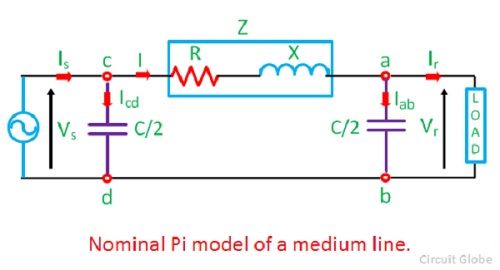
In the nominal pi model of a medium transmission line, the series impedance of the line is concentrated at the centre and half of each capacitance is placed at the centre of the line. The nominal Pi model of the line is shown in the diagram below.
 In this circuit,
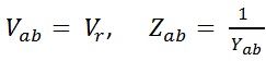 By Ohm’s law
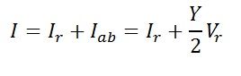
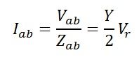 By KCL at node a,
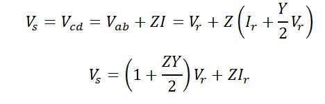
 Voltage at the sending end
By ohm’s law
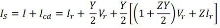
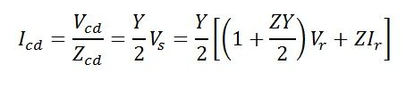 Sending-end current is found by applying KCL at node c
or
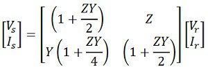
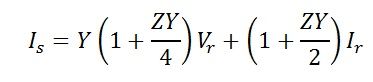 Equations can be written in matrix form as
Also,
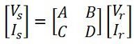
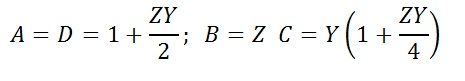
Hence, the ABCD constants for nominal pi-circuit model of a medium line are
 Phasor diagram of nominal pi model
The phasor diagram of a nominal pi-circuit is shown in the figure below.
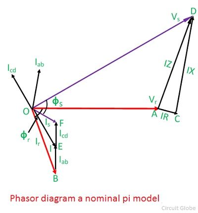 It is also drawn for a lagging power factor of the load. In the phasor diagram the quantities shown are as follows;
OA = Vr – receiving end voltage. It is taken as reference phasor.
OB = Ir – load current lagging Vr by an angle ∅r.
BE = Iab – current in receiving-end capacitance. It leads Vr by 90°.
The line current I is the phasor sum of Ir and Iab. It is shown by OE in the diagram.
AC = IR – voltage drop in the resistance of the line. It is parallel to I.
CD = IX -inductive voltage drop in the line. It is perpendicular to I.
AD = IZ – voltage drop in the line impedance.
OD = Vs – sending–end voltage to neutral. It is phasor sum of Vr and IZ.
The current taken by the capacitance at the sending end is Icd. It leads the sending–end voltage Vs by 90
OF = Is – the sending–end current. It is the phasor sum of I and Icd.
∅s – phase angle between Vs and Is at the sending end, and cos∅s will give the sending-end power factor.
Explanation super